OEE model
In the OEE model the capturability of values as well as the identification of capturable values is indicated by the adjectives “actual”, “ideal”, and “potential” in the respective terms. “Actual” quantities are real quantities and can be measured. “Potential” key figures cannot be measured at the machine, but can be derived from planning values of the organization. “Ideal” values, on the other hand, must be calculated and cannot be recorded directly.
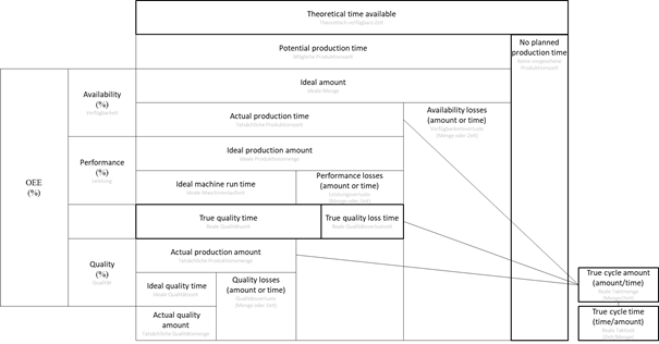
The model represents the view on quantity as well as on time in one diagram. To make this clear to the observer, the terms end with “Amount/amount” or “Time/time”. If terms do not have these endings or if there is a special case, as with the ideal cycles, round brackets indicate whether the term refers to the quantity, time, quantity and time, or a ratio. Ratios will be indicated in terms of quantity per time, time per quantity, or percentage. The exact specification of units for quantity and time was deliberately dispensed in order to further underline the generic applicability. To show that the relationship to quantity or time is ultimately irrelevant, corresponding terms are linked with the following symbol:

This allows a generic application at many different companies as different machine measurement data can be used. The conversion takes place with the help of the Ideal Cycle Amount or Ideal Cycle Time, which is explained in Calculation logic & variables. All quantities described as not ideal thus refer to the real machine and can therefore also be measured directly or indirectly.
Calculation logic & variables
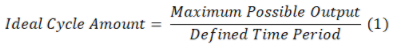
Ideal Cycle Amount and Ideal Cycle Time (1), (2), (3)
The Ideal Cycle Amount describes the maximum quantity that can be applied within a certain period of time, see formula (1). This value can only be achieved by an ideal machine, therefore the cycle quantity is described as ideal. This applies to all sizes described as ideal.
Its counterpart represents the Ideal Cycle Time, see formula (2).
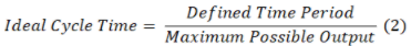
The quantities can be converted into each other by simply applying the exponent “-1”.

Potential Production Time (4)
The Potential Production Time describes the period of time in which production is planned for the machine. This production time is given the adjective “potential” and not “ideal”, since the organization defines it as a possible time period for production without any direct connection to the ideal machine.

Ideal Amount (5)
The Ideal Amount describes the maximum possible quantity to be produced within the Possible Production Time, see formula (5).

Actual Production Time (APT) (6)
The Actual Production Time describes the actual time period during which the machine produces products, regardless of speed or quality. In this respect, the adjective “actual” is added to this variable to make it easier to understand (this also applies to the following variables). Since Availability Losses, see below, prevent production the Actual Production Time is always shorter than the Potential Production Time, unless it is an ideal machine.

The Actual Production Time can also be represented as a quantitative figure, the Ideal Production Amount, see formula (7), (8) or (9).
Ideal Production Amount (7), (8), (9)
The Ideal Production Amount describes the amount that an ideal machine running at maximum speed could have produced within the Actual Production Time.

The calculation of the Actual Production Time explained above was carried out on the basis of a time reference. The same calculation is also possible with a quantity reference; for example, the Ideal Production Amount could also be calculated directly with the Ideal Amount minus the Availability Losses (amount).

It is also possible to calculate the Ideal Production Amount on the basis of the Potential Production Time, since the Potential Production Time and the Ideal Amount, as shown in the diagram, are equivalent to each other.

Thus it is shown that many possible ways of calculation exist to obtain equivalent values. For reasons of clarity, the following calculations are only given under respect to a time reference and not showing all possible calculation paths.
Ideal Machine Runtime (10)
The Ideal Machine Runtime describes the time it would have taken for an ideal machine to produce the Actual Production Amount at maximum speed.

As the diagram shows, the Ideal Machine Runtime can also be represented as Actual Production Amount.
Actual Production Amount (APA) (11)
The Actual Production Amount reflects the products manufactured in reality within the Actual Production Time and Possible Production Time.

Ideal Quality Time (12)
The Ideal Quality Time is calculated by subtracting the Quality Losses from the Ideal Machine Runtime, see Losses. It reflects the time that an ideal machine, which ultimately only produces good parts, would have needed to produce the Actual Quality Amount.

Actual Quality Amount (13)
The Actual Quality Amount reflects the produced good parts. It is also calculated using the Ideal Cycle Amount.

Availability (14)
Availability can be represented either by the ratio of Actual Production Time to Potential Production Time, or by the ratio of Ideal Production Amount to Ideal Amount. This results in a percentage value for Availability, which must be less than 100% if the machine is not ideal.

Performance (15)
The Performance can be calculated either from the ratio of Ideal Machine Runtime to Actual Production Time or Actual Production Amount to Ideal Production Amount. This also results in a percentage value for the activity. If it is not an ideal machine, it must be less than 100%.

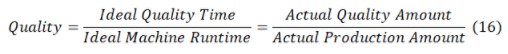
Quality (16)
The Quality can either be calculated from the ratio of Ideal Quality Time to Ideal Machine Runtime or Actual Quality Amount to Actual Production Amount. This results in a percentage value for the Quality, which, if it is not an ideal machine, must be less than 100%.
OEE (17)
The OEE is calculated using the following formula:

Losses
Availability Losses
For Availability Losses, we recommend you to record unplanned downtimes such as malfunctions, delays, line restrictions and, if necessary, planned downtimes such as maintenance, inspection, cleaning, repair and setup, conversion or format change. However, you define the exact definition when matching the individual parameters. A direct allocation of the losses to the cause is not necessary for the calculation.
The special aspect of Availability Losses is that they can be recorded and measured time-wise through machine data. With regard to the quantity, they can only be calculated using the Ideal Cycle Amount. This is simply due to the fact that non-produced ideal amounts cannot be measured either.
Performance Losses
Performance Losses reflect a reduced production speed and can include short stoppages. You can decide for yourself whether you want to record short stoppages or not, this can be set when matching the parameters. If you have specified that short stoppages must be recorded, you must define a time period for this. For example, you can define that Availability Losses (time) shorter than 20 seconds are no longer counted as Availability Losses (time), but instead as Performance Losses (time). Availability Losses (time) shorter than 20 seconds, are then deducted from the Availability Losses and added to the Performance Losses (time) and the Actual Production Time.
Of course, this also applies correspondingly to the Availability Losses (amount) and Performance Losses (amount) and the Ideal Production Amount.
This calculation of the short stoppages takes place between the matching of the machine data and the creation of the OEE input variables. For example, it becomes difficult when there is an interval boundary between a machine-down event and a machine-up event, a kind of standstill that counts as a loss of availability. It is now necessary to check whether the total downtime lasts less than 20 seconds, regardless of the interval limit. Thus, a short stoppage for the penultimate interval can only be identified with certainty if the last interval is already greater than or equal to 20 seconds, or if a machine-up event has already occurred previously.
The special feature of Performance Losses is that they are not measured directly. They must always be calculated.
Quality Losses
We recommend you to define Quality Losses in such a way that they include all products that do not immediately meet the required quality requirements. The Quality Losses can be recorded quantitatively.
Splitting
The term “Splitting” describes the allocation of machine data to the OEE input parameters. This sections shows examples which explain the methodology used.
Input variable calculation - Example 1
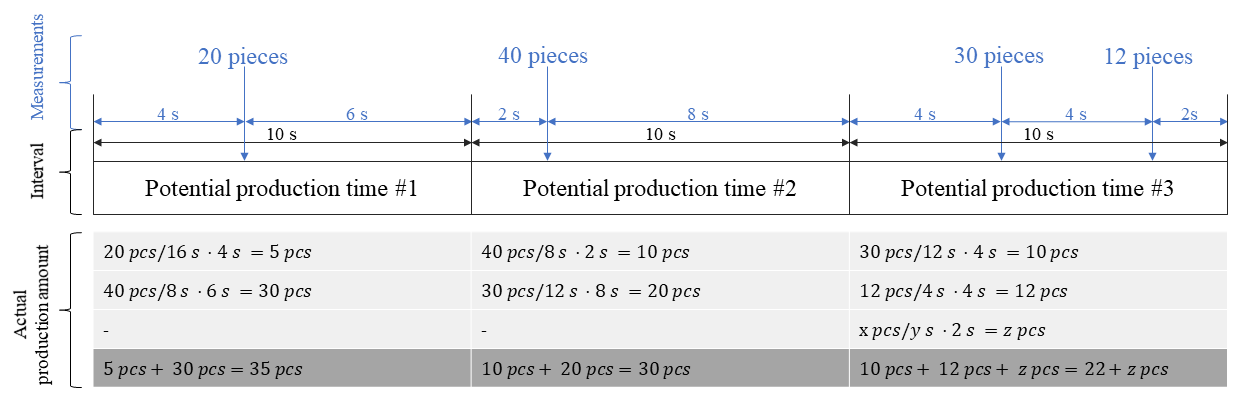
It is crucial for the OEE application to correctly allocate the input data to the corresponding intervals of the Possible Production Time or resolution time. This allocation is explained below using an example with reference to the data in the Machine dashboard. Within three intervals of the Possible Production Time, the machine sends four measured values (shown in blue), which indicate the number of products since the last measured value, that is, the actual production quantity.
The first measured value is 20 pieces. The previous measured value was 16 seconds ago, outside the display range. Thus it is proportionally taken into account to 25% of the first interval. With the same logic, 75% of the second measured value is calculated for the first interval. The total of the proportional allocation results in the actual production quantity for the first interval of 35 pieces. This results in a value of 30 pieces for the second interval. In this example, measured value number four is the most recent measured value sent by the machine. To be able to calculate the actual production quantity for the third interval, you must wait for the next measured value “z”, which is received after “y” seconds.
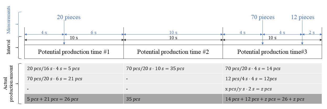
Input variable calculation - Example 2
If no measurement is received within an interval the next measurement will be calculated proportionally. The Actual Production Amount for the second interval will therefore be 35 pieces even if there was no measurement received.
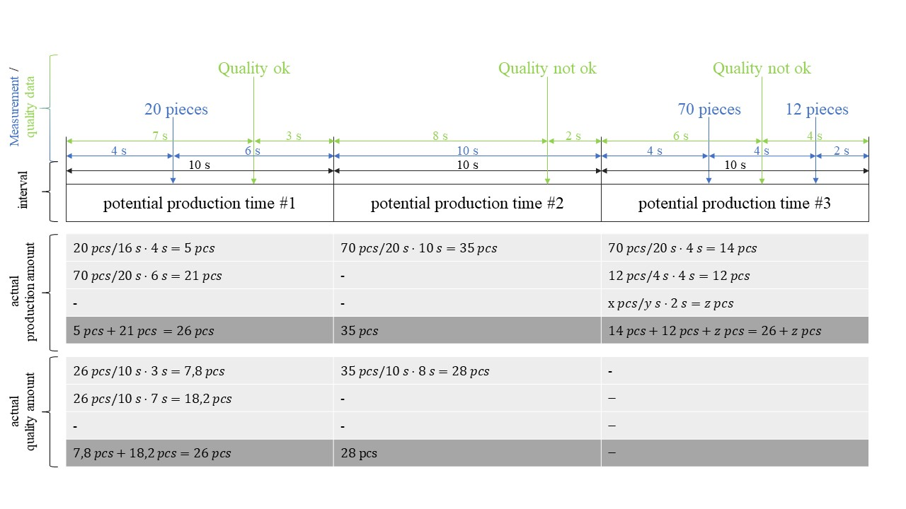
Input variable calculation - Example 3
The calculation of the quality looks more complex, since the quality data does not necessarily come to the same point as the corresponding measured value. Quality data or quality data derived from measurements can occur irregularly.
In contrast to the measurement of produced amount of pieces, the quality data refers to the future period. The last quality status before the first interval was OK, so the entire quantity of the first interval is taken into account as quality amount. Since the quality in interval one is OK from second six onwards, the quality in the second interval is also OK for the first eight seconds. This is not the case for the last two seconds. In interval two, 80% of the quantity actually produced corresponds to the quality requirements, that is, 28 pieces.
Of course, these calculations do not reflect reality to 100%, since the assumption is made that production will be uniform. This is more probable in process manufacturing than in discrete manufacturing, since several workpieces can be produced at once per operation. A better representation can be achieved by using data from the digital workpiece. In this case, the quality data is directly assigned to the workpiece and each workpiece is recorded individually.
Input variables for the OEE calculation
In the OEE application you can select different calculation methods that require different input variables.
A total of 5 out of 7 input variables are required to calculate the OEE.
The following table shows the input variables and the relationship to the different calculation models, explained below:
| Input variables | Description | Reference Point | Model PPQ/1 | Model PQL/2 | Model PPL/3 | Model LPQ/4 | Model LQL/5 | Model LPL/6 |
|---|---|---|---|---|---|---|---|---|
| Ideal Cycle Amount | Ideal production speed | Link to the production plan or manual entry in the application | x | x | x | x | x | x |
| Potential Production Time | The period in which the machine is scheduled for production. | Link to shift plan or manual entry in the application | x | x | x | x | x | x |
| Actual Production Time | Describes the time period during which the machine is actually running and producing products, regardless of speed or quality. Since Availability Losses prevent production, the Actual Production Time, unless it is an ideal machine, is always shorter than the Possible Production Time. | Automatic reference | x | x | x | |||
| Availability Losses | For Availability Losses, it is recommended to record unplanned downtimes such as malfunctions, maintenance, line restrictions and, if necessary, planned downtimes such as maintenance, inspection, cleaning, repair and equipping, modification or format change. | Automatic reference | x | x | x | |||
| Actual Production Amount | Reflects the products manufactured in reality within the Actual Production Time and Possible Production Time. | Automatic reference | x | x | x | x | ||
| Quality Losses | It is recommended to define Quality Losses in such a way that they include all products that do not immediately meet the required quality requirements, including rework, B-goods and start-up losses. The Quality Losses are concentrated on the parts produced by the plant and their quality and can be recorded quantitatively. | Automatic reference | x | x | x | x | ||
| Actual Quality Amount | The quality quantity is therefore calculated as follows: Actual Quality Amount = Actual Production Amount - Quality Losses (amount). | Automatic reference | x | x | x | x |
Calculation pathways
The following image explains the naming conventions of the pathways. The same terminology is used in the Computation section when creating a new profile, see Administration > Creating machine profiles > Computation.
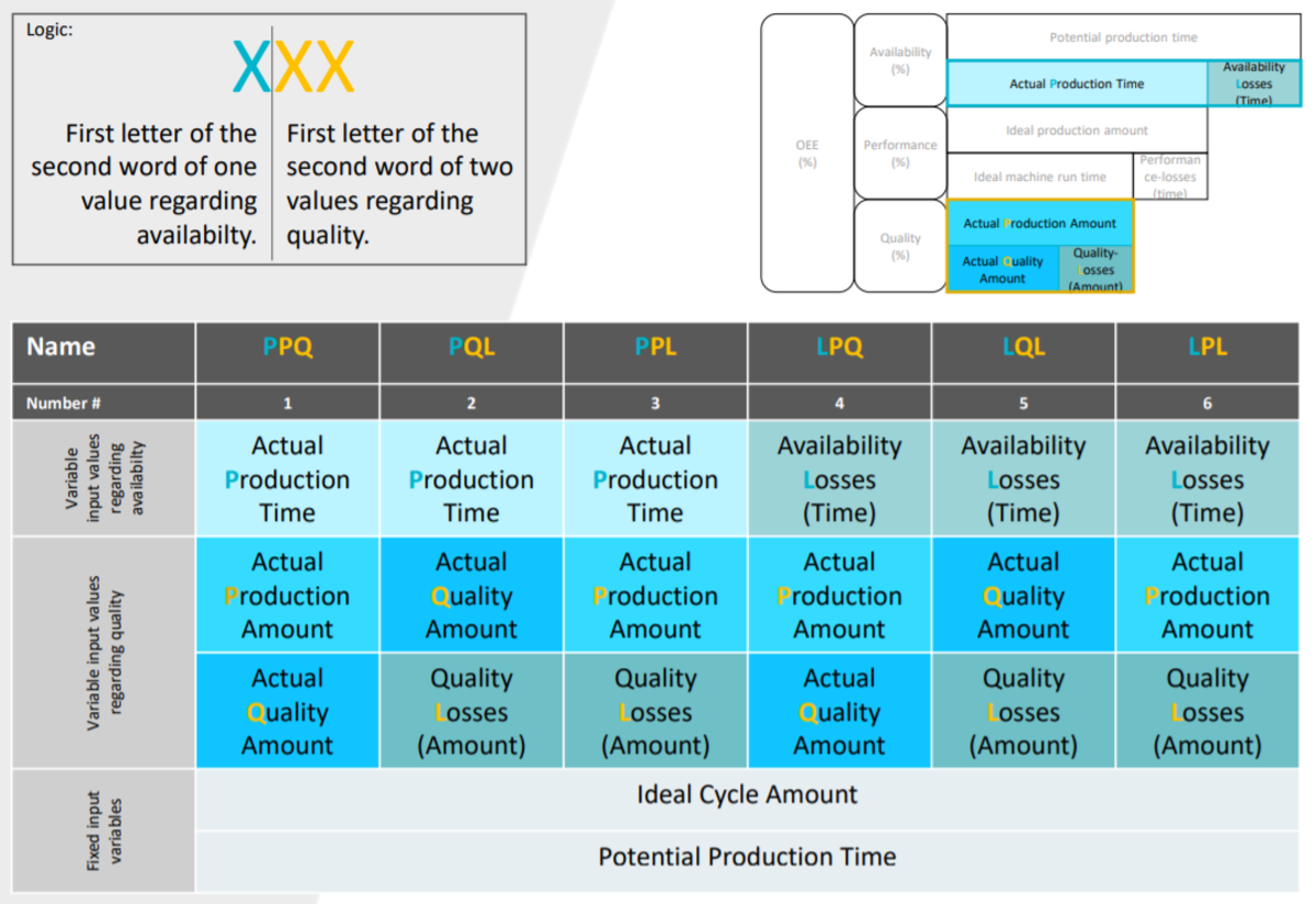
In the following, details on each calculation pathway are provided.
Info
The tables at the top show which variables, starting from the input variables, are needed to calculate all other variables including the OEE. The different colors used in the images are used only for better understanding and clarity. Below the image you find the corresponding formulas. The formulas which are necessary to calculate the OEE are marked in italics in the table.
Calculation pathway #1
| Input Variables | Variables needed for calculation pathway |
|---|---|
| Ideal Cycle Amount | x |
| Potential Production Time | x |
| Actual Production Time | x |
| Availability Losses (Time) | |
| Actual Production Amount | x |
| Actual Quality Amount | x |
| Quality Losses (Amount) |
This overview shows which variables are needed to calculate each variable, including the OEE. The formulas marked in italics in the table below are necessary to calculate the OEE.
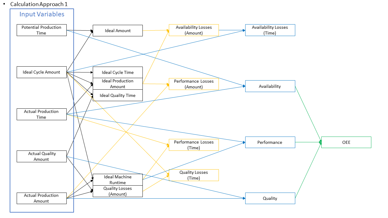
| 1. | Ideal Amount = Potential Production Time x Ideal Cycle Time |
| 2. | Ideal Cycle Time = Ideal Cycle Amount-1 |
| 3. | Ideal Production Amount = Actual Production Time x Ideal Cycle Amount |
| 4. | Ideal Quality Time = Actual Quality Amount x Ideal Cycle Amount-1 |
| 5. | Ideal Machine Runtime = Actual Production Amount x Ideal Cycle Amount-1 |
| 6. | Quality Losses (Amount) = Actual Production Amount - Actual Quality Amount |
| 7. | Availability Loses (Amount) = Ideal Amount - Ideal Production Amount |
| 8. | Performance Losses (Amount) = Ideal Production Amount - Actual Production Amount |
| 9. | Performance Losses (Time) = Actual Production Time - Ideal Machine Runtime |
| 10. | Quality Losses (Time) = Quality Losses (Amount) x Ideal Cycle Amount-1 |
| 11. | Availability Losses (Time) = Availability Losses (Amount) x Ideal Cycle Amount-1 |
| 12. |
Availability = |
| 13. | Performance = Ideal Machine Runtime ⁄ Actual Production Time |
| 14. | Quality = Actual Quality Amount ⁄ Actual Production Amount |
| 15. | OEE = Availability x Performance x Quality |
Calculation pathway #2
| Input Variables | Variables needed for calculation pathway |
|---|---|
| Ideal Cycle Amount | x |
| Potential Production Time | x |
| Actual Production Time | x |
| Availability Losses (Time) | |
| Actual Production Amount | |
| Actual Quality Amount | x |
| Quality Losses (Amount) | x |
This overview shows which variables are needed to calculate each variable, including the OEE. The formulas marked in italics in the table below are necessary to calculate the OEE.
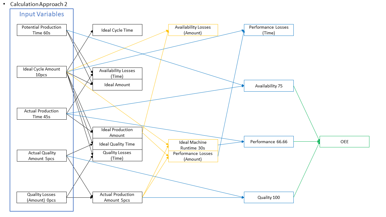
| 1. | Ideal Cycle Time = Ideal Cycle Amount-1 |
| 2. | Availability Losses (Amount) = Potential Production Time - Actual Production Time |
| 3. | Ideal Amount = Potential Production Time x Ideal Cycle Amount |
| 4. | Ideal Production Amount = Actual Production Time x Ideal Cycle Amount |
| 5. | Ideal Quality Time = Actual Production Amount x Ideal Cycle Amount-1 |
| 6. | Quality Losses (Time) = Quality Losses (Amount) x Ideal Cycle Amount-1 |
| 7. | Actual Production Amount = Actual Quality Amount + Quality Losses (Amount) |
| 8. | Performance Losses (Amount) = Performance Losses (Time) x Ideal Cycle Amount |
| 9. | Ideal Machine Runtime = Actual Production Amount x Ideal Cycle Amount-1 |
| 10. | Performance Losses (Amount) = Ideal Production Amount - Actual Production Amount |
| 11. | Performance Losses (Time) = Availability Losses (Amount) x Ideal Cycle Amount-1 |
| 12. |
Availability = |
| 13. | Performance = Ideal Machine Runtime ⁄ Actual Production Time |
| 14. | Quality = Actual Quality Amount ⁄ Actual Production Amount |
| 15. | OEE = Availability x Performance x Quality |
Calculation pathway #3
| Input Variables | Variables needed for calculation pathway |
|---|---|
| Ideal Cycle Amount | x |
| Potential Production Time | x |
| Actual Production Time | x |
| Availability Losses (Time) | |
| Actual Production Amount | x |
| Actual Quality Amount | |
| Quality Losses (Amount) | x |
This overview shows which variables are needed to calculate each variable, including the OEE. The formulas marked in italics in the table below are necessary to calculate the OEE.
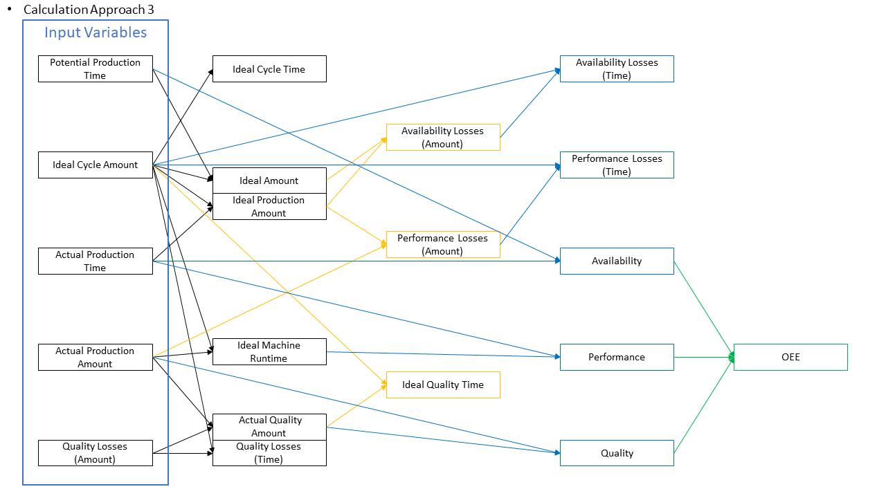
| 1. | Ideal Cycle Time = Ideal Cycle Amount-1 |
| 2. | Ideal Amount = Potential Production Time x Ideal Cycle Amount |
| 3. | Ideal Production Amount = Actual Production Time x Ideal Cycle Amount |
| 4. | Ideal Machine Runtime = Actual Production Time x Ideal Cycle Amount-1 |
| 5. | Actual Quality Amount = Actual Production Amount - Quality Losses (Amount) |
| 6. | Quality Losses (Time) = Quality Losses (Amount) x Ideal Cycle Amount-1 |
| 7. | Performance Losses (Amount) = Ideal Amount + Ideal Production Amount |
| 8. | Performance Losses (Amount) = Ideal Production Amount - Actual Production Amount |
| 9. | Ideal Quality Time = Actual Quality Amount x Ideal Cycle Amount-1 |
| 10. | Availability Losses (Time) = Availability Losses (Amount) - Ideal Cycle Amount-1 |
| 11. | Performance Losses (Time) = Performance Losses (Amount) x Ideal Cycle Amount-1 |
| 12. |
Availability = |
| 13. | Performance = Ideal Machine Runtime ⁄ Actual Production Time |
| 14. | Quality = Actual Quality Amount ⁄ Actual Production Amount |
| 15. | OEE = Availability x Performance x Quality |
Calculation pathway #4
| Input Variables | Variables needed for calculation pathway |
|---|---|
| Ideal Cycle Amount | x |
| Potential Production Time | x |
| Actual Production Time | |
| Availability Losses (Time) | x |
| Actual Production Amount | x |
| Actual Quality Amount | x |
| Quality Losses (Amount) |
This overview shows which variables are needed to calculate each variable, including the OEE. The formulas marked in italics in the table below are necessary to calculate the OEE.
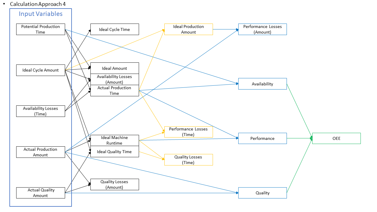
| 1. | Ideal Cycle Time = Ideal Cycle Amount-1 |
| 2. | Ideal Amount = Potential Production Time x Ideal Cycle Amount |
| 3. | Availability Losses (Amount) = Availability Losses (Time) x Ideal Cycle Amount |
| 4. | Actual Production Time = Potential Production Time - Availability Losses (Time) |
| 5. | Ideal Machine Runtime = Actual Production Amount - Ideal Cycle Amount-1 |
| 6. | Ideal Quality Time = Actual Quality Amount x Ideal Cycle Amount-1 |
| 7. | Quality Losses (Amount) = Actual Production Amount - Actual Quality Amount |
| 8. | Ideal Production Amount = Actual Production Amount x Ideal Cycle Amount |
| 9. | Performance Losses (Time) = Actual Production Time - Ideal Machine Runtime |
| 10. | Quality Losses (Time) = Ideal Machine Runtime - Ideal Quality Time |
| 11. | Performance Losses (Time) = Ideal Production Amount x Actual Production Amount |
| 12. |
Availability = |
| 13. | Performance = Ideal Machine Runtime ⁄ Actual Production Time |
| 14. | Quality = Actual Quality Amount ⁄ Actual Production Amount |
| 15. | OEE = Availability x Performance x Quality |
Calculation pathway #5
| Input Variables | Variables needed for calculation pathway |
|---|---|
| Ideal Cycle Amount | x |
| Potential Production Time | x |
| Actual Production Time | |
| Availability Losses (Time) | x |
| Actual Production Amount | |
| Actual Quality Amount | x |
| Quality Losses (Amount) | x |
This overview shows which variables are needed to calculate each variable, including the OEE. The formulas marked in italics in the table below are necessary to calculate the OEE.
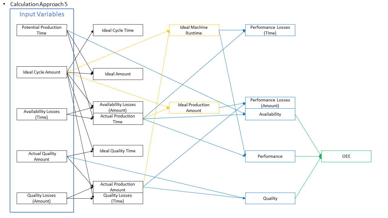
| 1. | Ideal Cycle Time = Ideal Cycle Amount-1 |
| 2. | Ideal Amount = Potential Production Time x Ideal Cycle Amount |
| 3. | Availability Losses (Amount) = Availability Losses (Time) x Ideal Cycle Amount |
| 4. | Actual Production Time = Potential Production Time - Availability Losses (Time) |
| 5. | Ideal Quality Time = Actual Quality Amount x Ideal Cycle Amount-1 |
| 6. | Actual Production Amount = Actual Quality Amount + Quality Losses (Amount) |
| 7. | Quality Losses (Amount) = Quality Losses (Amount) x Ideal Cycle Amount-1 |
| 8. | Ideal Machine Runtime = Actual Production Amount x Ideal Cycle Amount-1 |
| 9. | Ideal Production Amount = Actual Production Time x Ideal Cycle Amount |
| 10. | Performance Losses (Time) = Actual Production Time - Ideal Machine Runtime |
| 11. | Performance Losses (Amount) = Ideal Production Amount - Actual Production Amount |
| 12. |
Availability = |
| 13. | Performance = Ideal Machine Runtime ⁄ Actual Production Time |
| 14. | Quality = Actual Quality Amount ⁄ Actual Production Amount |
| 15. | OEE = Availability x Performance x Quality |
Calculation pathway #6
| Input Variables | Variables needed for calculation pathway |
|---|---|
| Ideal Cycle Amount | x |
| Potential Production Time | x |
| Actual Production Time | |
| Availability Losses (Time) | x |
| Actual Production Amount | x |
| Actual Quality Amount | |
| Quality Losses (Amount) | x |
This overview shows which variables are needed to calculate each variable, including the OEE. The formulas marked in italics in the table below are necessary to calculate the OEE.
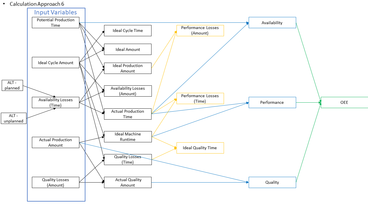
| 1. | Ideal Cycle Time = Ideal Cycle Amount-1 |
| 2. | Ideal Amount = Potential Production Time x Ideal Cycle Amount |
| 3. | Availability Losses (Amount) = Availability Losses (Time) x Ideal Cycle Amount |
| 4. | Actual Production Time = Potential Production Time - Availability Losses (Time) |
| 5. | Ideal Machine Runtime = Actual Production Amount x Ideal Cycle Amount-1 |
| 6. | Quality Losses (Time) = Quality Losses (Time) x Ideal Cycle Time-1 |
| 7. | Actual Quality Amount (Amount) = Actual Production Amount - Quality Losses (Amount) |
| 8. | Ideal Production Amount = Ideal Amount - Availability Losses (Amount) |
| 9. | Performance Losses (Time) = Actual Production Time - Ideal Machine Runtime |
| 10. | Ideal Quality Time = Ideal Machine Runtime - Quality Losses (Time) |
| 11. | Performance Losses (Amount) = Ideal Production Amount - Actual Production Amount |
| 12. |
Availability = |
| 13. | Performance = Ideal Machine Runtime ⁄ Actual Production Time |
| 14. | Quality = Actual Quality Amount ⁄ Actual Production Amount |
| 15. | OEE = Availability x Performance x Quality |