Overview
Casting is a manufacturing process in which a liquid material is usually poured into a mould, which contains a hollow cavity of the desired shape, and then is allowed to solidify.
A casting defect is an undesired irregularity in a metal casting process. There are many types of defects in casting like blow holes, pinholes, burr, shrinkage defects, mould material defects, pouring metal defects, metallurgical defects, etc. Defects are an unwanted thing in the casting industry. For removing this defective product, all industry have their quality inspection department. But the main problem is that this inspection process is carried out manually. It is a very time-consuming process and due to human accuracy, this is not 100% accurate. This can lead to the rejection of the whole order which creates a big loss to the company.
Casting defect detection automates the inspection process by utilizing the power of deep learning algorithms.
For the purpose of showcasing this use case, we followed these steps:
- Download the open-source Kaggle dataset from https://www.kaggle.com/ravirajsinh45/real-life-industrial-dataset-of-casting-product.
- Method 1: Use MLW’s intuitive drag and drop Neural Network (NN) Designer to build your deep neural network architecture and start training the model.
- Method 2: Use MLW’s integrated Jupyter Notebook to train your model using the transfer learning approach.
- Use the transformed ONNX model, pre-processing, and post-processing scripts to build an inference pipeline and deploy the same to production (Cumulocity IoT Machine Learning).
- The pre-processing script tranforms the data to a valid format which the ONNX model accepts.
- The post-processing script assigns a proper class to the predicted probabilities.
- Make inferences using the model in production.
Prerequisites
Download the CastingDefectDetectionDemo.zip file which contains two folders as following:
- Method1
- Pre-processing and post-processing Python scripts (castingPreProcessingForNN.py and castingPostProcessingForNN.py)
- Test images (testDefectImage.png and testOkImage.png)
- Method2
- Pre-processing and post-processing Python scripts (castingPreProcessingForJNB.py and castingPostProcessingForJNB.py)
- Test images (testDefectImage.png and testOkImage.png)
- Jupyter Notebook (castingDefectDetectionDemo.ipynb)
Running the demo scripts requires:
- Prior experience with Python and understanding of the data science processes.
- Familiarity with Cumulocity IoT and its in-built apps.
- Subscription of the MLW, Zementis, ONNX microservices (10.7.0.x.x or higher) and the Machine Learning Workbench, Machine Learning applications on the tenant.
Casting defect detection
This section deals with the basic data science steps of creating a casting defect detection model using Machine Learning Workbench with the open-source Kaggle dataset. Follow the sections below for downloading data, building a neural network architecture, transfer learning with MobileNet, training the model, deploying the model to production and using the same to detect defects in the casts.
Collecting data from Kaggle
Download the open-source Kaggle dataset from https://www.kaggle.com/ravirajsinh45/real-life-industrial-dataset-of-casting-product.
Info: You will get two folders when you unzip the downloaded dataset. Use the casting_data folder and delete the casting_512x512 folder.
All the images provided with this dataset are the top view of the submersible pump impeller.
The dataset contains 7348 images in total. These are all grey-scaled images of the size 300x300 pixels. The augmentation is already applied in all the images.
There are mainly two categories:
- Defective
- Ok
For training a classification model, the data is split into training and testing folders. Both train and test folders contain def_front and ok_front subfolders.
- train: def_front has 3758 and ok_front has 2875 images
- test: def_front has 453 and ok_front has 262 images
Change the name of test folder to validation and create a ZIP file of these two folders (i.e. a ZIP file contaning train and validation folders).
Uploading the data to MLW
Log in to the MLW and use the Upload Resources option to upload the created ZIP file. This might take a few minutes depending on your internet bandwidth.
After the data is uploaded sucessfully, navigate to the Data folder of the MLW and click on the ZIP file. You should see the metadata of the uploaded dataset.
Training the model
Method 1: Creating a custom deep neural network architecture
-
Follow the steps described in Machine Learning Workbench > Neural Network (NN) Designer and create a new architecture file named castingModelDesigner.architecture with “None” as Architecture.
-
Select the castingModelDesigner.architecture file and click the edit icon
 to open an interface/editor to build your own deep neural network architecture by dragging and dropping various layers available in the menu at the left.
 -
Build a deep neural network architecture using the below example:
-
Save the architecture file and train the deep neural network model by setting the Training Parameters as below:
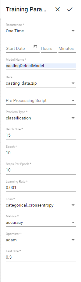
-
To monitor the model building progress, click Tasks in the navigator and click castingDefectModel. The training time is generally 30-50 minutes for 10 epochs for this particular dataset. Initially, the task status is INITIALISING and gets changed to TRAINING STARTED once the training starts.
After the training is complete, the task status will be set to COMPLETED and a model named castingDefectModel.onnx is saved to the Model folder.
Method 2: Training a model in Jupyter Notebook using the transfer learning technique with Mobilenet architecture
-
The CastingDefectDetectionDemo.zip has a folder named Method2 which contains a Jupyter Notebook file named castingDefectDetectionDemo.ipynb. Use the MLW’s upload functionality to upload the Notebook file.
-
In the Code folder of the MLW, click castingDefectDetectionDemo.ipynb to view the metadata of the file.
-
Click the edit icon
to open the Jupyter Notebook and execute all the cells in sequence.
Once all the cells are executed successfully, a model named castingDefectModelViaJNB.onnx is saved to the Model folder.
Deploying the model using the inference pipeline
Now that the model is successfully trained (by any of the above two training methods) and available for serving in the form of an ONNX file, you can create an inference pipeline for deploying the model to production.
The CastingDefectDetectionDemo.zip contains two folders namely Method1 and Method2. Depending on the training method used, upload the relevant Python scripts.
- If Method 1 is has been used for training: Use castingPreProcessingForNN.py and castingPostProcessingForNN.py Python scripts from the Method1 folder. Use the MLW’s upload functionality to upload these Python files.
- If Method 2 is has been used for training: Use castingPreProcessingForJNB.py and castingPostProcessingForJNB.py Python scripts from the Method2 folder. Use the MLW’s upload functionality to upload these Python files.
The inference pipeline uses a pre-processing script, a model (.onnx file) and a post-processing script.
- The pre-processing script is used to pre-process incoming test data (image) to convert it into 250250 size. The pre-processing script *castingPreProcessingForNN.py looks like below.
  import numpy as np
  from PIL import Image
  import io
  def process(content):
      im = Image.open(io.BytesIO(content))
      im = im.resize((250,250))
      x = np.array(im,dtype=np.float32)
      x = np.expand_dims(x,0)
      return {"Conv2D_input":x}
- The post-processing script is used to assign proper classes to the predicted probabilities from the ONNX model. The post-processing script castingPostProcessingForNN.py looks like below.
  def process(content):
      import numpy as np
      classes = ["defective","ok"]
      cla = classes[np.argmax(content[0])]
      return {"Dense":content[0].tolist(),"PredictedClass":cla}
-
Follow the steps described in Machine Learning Workbench > Inference pipeline and create an inference pipeline named castingPipeline.pipeline by selecting ‘castingDefectModel.onnx’ or ‘castingDefectModelViaJNB.onnx’ as Model, ‘castingPreProcessingForNN.py’ as Pre-processing Script and ‘castingPostProcessingForNN.py’ as Post-processing Script .
This creates a new pipeline file named castingPipeline.pipeline in the Inference Pipeline folder. you will be able to see the metadata of the pipeline file by clicking on it.
-
Deploy the pipeline to the production.
Predictions using the deployed pipeline
Now that the inference pipeline is successfully deployed to production and available for serving, you can make predictions using the test data.
-
The CastingDefectDetectionDemo.zip contains two folders namely Method1 and Method2. Both the folders contain testDefectImage.PNG and testOkImage.PNG test images. Use the MLW’s upload functionality to upload these test image files from any of the folders.
-
Navigate to the Data folder and select testDefectImage.PNG. Predict the class of image using castingPipeline.
The predictions file will be stored in the Data folder with the name testDefectImage_timeStamp.json. Edit the predictions JSON file to view the predictions.